3D Tracking in Braid

Principle of operation

This page describes the basic principles of how tracking in 3D is implemented by Braid. A more detailed and more mathematical description can be found in the paper describing Braid's predecessor, Straw et al. (2011). Please refer to this for more details.

Straw et al. 2011: Straw AD, Branson K, Neumann TR, Dickinson MH (2011) Multicamera Realtime 3D Tracking of Multiple Flying Animals. Journal of The Royal Society Interface 8(11), 395-409. doi:10.1098/rsif.2010.0230

.

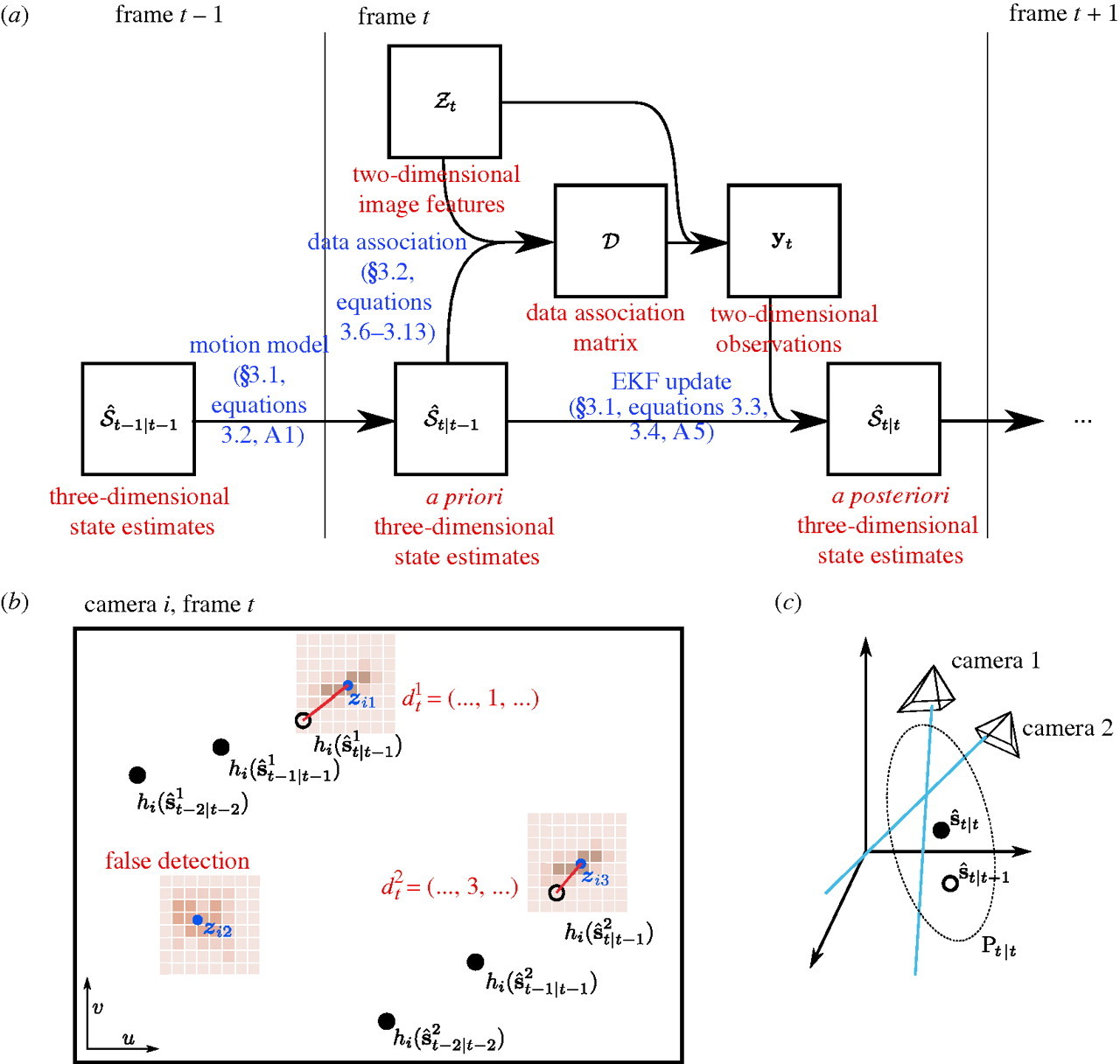
Figure 1: Principles of 3D Tracking in Braid. References in blue refer to parts of Straw et al. (2011). (a) Flowchart of operations. (b) Schematic of a two-dimensional camera view showing the raw images (brown), feature extraction (blue), state estimation (black), and data association (red). (c) Three-dimensional reconstruction using the EKF uses prior state estimates (open circle) and observations (blue lines) to construct a posterior state estimate (filled circle) and covariance ellipsoid (dotted ellipse). This figure and some caption text reproduced from Figure 2 of Straw et al. (2011) under the Creative Commons Attribution License.

(TODO: walkthrough of figure above.)

Tracking in water with cameras out of water

One important aspect of Braid not covered in Straw et al. (2011) is the the capability of tracking fish (or other objects in water) from cameras placed above the water surface.

Refraction

When looking through the air-water interface (or any refractive boundary), objects on the other side appear from a different direction than the direct path to the object due to refraction. Mathematically, refraction is described by Fermat's principle of least time, and this forms the basis of Braid's tracking in water.

Principle of operation for tracking in water

When considering the principle of operation of 3D tracking described above, the primary addition to Braid required for tracking in water is the ability to model the rays coming from the animal to the camera not as straight lines but rather having a bend due to refraction. To implement this, the observation model of the extended Kalman filter is extended to incorporate the air-water boundary so that it consists of both a 3D camera model and air-water surface model. Thus, during the update step of the Kalman filter, this non-linear model is linearized about the expected (a priori) position of the tracked object.

Currently, Braid has a simplification that the model of the air-water boundary is always fixed at z=0. Thus, anything with z<0 is under water and anything with z>0 is above water. This implies that the coordinate frame for tracking with an air-water boundary must have this boundary at z=0 for correct tracking.

How to enable tracking in water.

Practically speaking, tracking using the model of an air-water boundary is enabled by placing the string <water>1.333</water> the XML camera calibration file. This will automatically utilize the refractive boundary model described above with a value for the refractive index of 1.333 for the medium at z<0. As 1.333 is the refractive index of water, it is a model of refraction in water.

Tracking multiple objects in 3D

It is possible to use Braid to track two or more objects in 3D. Typically this requires the per-camera, 2D object detection to be set to also detect multiple objects. Thus, the parameter max_num_points in the Object Detection configuration of Strand Camera should be set to at least the number of objects that should be tracked.

To maintain object identity over time, such that a single trajectory is recorded for a single animal, Braid uses a simple data association algorithm which assumes independent movement of the tracked objects. This is sufficient in many cases for tracking animals even when they interact strongly with each other, but it is typically be necessary to tune relevant tracking and data association parameters to get the best performance possible.

Details about how data are processed online and saved for later analysis

While running, Braid saves a copy of all incoming feature detections from the cameras as a first step prior to inspecting frame numbers and bundling data from synchronously acquired data from multiple cameras. Combined with issues such as unreliable networks, this has the unfortunate effect that frames saved to disk cannot be guaranteed to be monotonically increasing. For online processing to implement 3D tracking, there is always an idea of "current frame number". Any data from prior frames is immediately discarded from further consideration (but it was saved to disk as described above). If the incoming frame number is larger than the current frame number, any accumulated data for the "current frame" is deemed complete and this is bundled for immediate processing. If the incoming frame number is larger than a single frame from the current frame number, additional frames of empty data are generated so that the stream of bundled data is contiguous (with no gaps) up until the incoming frame number, which then becomes the new "current frame number".

Note that in post-processing based on data saved in .braidz files, a better reconstruction can be made than possible in the online approach described above because data which may have been discarded originally could be incorporated into the tracking process. Furthermore, because latency is no longer a significant concern, reconstruction for a particular instant need not be performed with only historical data but can also incorporate information that occurred after that instant.